Normal Distribution 101

This is a bell curve. An inverted U, where the right side is a mirror image of the left side. To place this mathematically, normal distribution is a continuous probability distribution which is symmetrical on both sides of the mean. However, skewed distributions can tilt on either side of the curve. Bell curves are formed by taking the average of a data set and then plotting those values around their mean on a sheet

Before we jump into understanding bell curves further, let’s revise what we call as a standard deviation. SD (σ) is nothing but the dispersion of a dataset from its average value. A stock with an opening and closing price of 50 and 120 (mean is say around 84) would be said to have higher σ than the equally priced stock with OP and CP as 80 and 90. More volatile stocks have higher σ

Coming back.

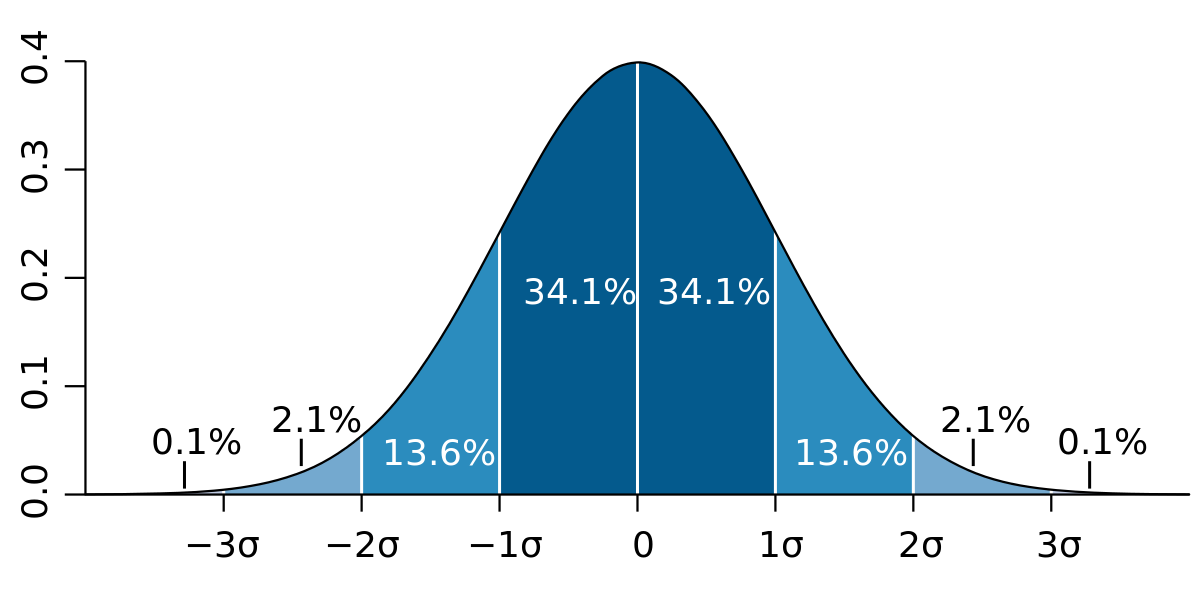
Bell curves are widely used in statistics, business and in markets. Some common examples would be the distribution on heights of people, returns on stocks, grades in an exam and your salaries. Let’s say that the average price of RIL stock across 2020 has been INR 1600 with a standard deviation of INR 30 daily. What are the chances that the stock would be between ₹1570 and ₹1630 on any random day in 2020? A: ~68% basis the table below

So, that’s the primer on bell curves.

Now, bell curves are pretty common and it’s a high possibility that you were already aware of them. However, bell curves are extremely important in understanding tail risks. Tail risks are the numbers that we usually ignore but should NEVER. Anyone willing to start a business or invest in markets should be aware of the inherent tail risks. Just keep this refresher on normal distribution handy for we will discuss them bad tail risks in our next thread

Goodbye!